Chapter 15 — Case Study 9 — Monte Carlo Measurement Uncertainty & Risk of Non-Compliance
🗺️ Chapter roadmap
- 0️⃣ Monte Carlo foundation (implicit in all case studies)
- 1️⃣ Why measurement uncertainty matters in GMP
- 2️⃣ True value vs measured value
- 3️⃣ Monte Carlo model: process variability + measurement uncertainty
- 4️⃣ Practical R simulation (risk of False Acceptance / False Non-Compliance)
- 5️⃣ GMP interpretation and regulatory context
🎯 Why This Matters
In pharmaceutical Quality Control, measurement uncertainty (MU) is usually documented in method validation reports, but rarely quantified in batch disposition decisions.
💡 Why QC laboratories rarely estimate measurement uncertainty for each batch
In routine pharmaceutical QC, only one (or at most two) determinations are usually performed for each batch where “one (or two) determinations per batch” refers, in practice, to each analytical parameter (e.g., assay, water content, pH, impurities).
Because statistical uncertainty requires replicate measurements, the uncertainty associated with the actual result obtained for that specific batch cannot be empirically estimated.
Laboratories therefore rely on an uncertainty value derived from method validation (repeatability, intermediate precision, recovery studies, etc.).
This value reflects the long-term performance of the analytical method but does not capture the measurement conditions of the current batch — such as analyst-to-analyst variability, instrument drift, sample matrix effects, or day-to-day operational factors.
Monte Carlo simulation provides a practical and GMP-compliant way to bridge this gap by integrating both process variability and method uncertainty into a quantitative risk estimate for a process operated under given capability and measurement uncertainty.
Importantly, Monte Carlo simulation does not estimate the uncertainty of the single measurement itself.
The following box explains how Monte Carlo integrates method uncertainty and process behaviour when only one QC measurement is available.
What Monte Carlo quantifies in this case
Monte Carlo simulation does
not estimate the uncertainty of the single QC measurement performed on a batch, as this would require replicate determinations.
Instead, it quantifies the
decision risk of batch misclassification by generating many plausible pairs of:
- the true batch value Xt, modeled from historical process variability or prior capability knowledge,
- the measured QC value Xm = Xt + ε, where the measurement error ε ~ N(0, u²) represents the method-validated standard uncertainty u.
The simulation then estimates the two
decision risks:
\[P(\mathrm{FNC}) = \frac{\mathrm{count}(X_m > \mathrm{USL} \land X_t \le \mathrm{USL})}{N}\]
\[P(\mathrm{FA}) = P\left(X_m \le \mathrm{USL} \mid X_t > \mathrm{USL}\right)\]
Yet, whenever a batch result is close to a specification limit, MU determines:
- the risk of False Non-Compliance (rejecting a good batch), and
- the risk of False Acceptance (releasing a batch whose true value is out of specification).
Monte Carlo simulation provides a simple and transparent way to quantify these risks using the fundamental relationship:
\[X_m = X_t + \varepsilon\]
where:
- $X_m$ = measured value
- $X_t$ = true (unknown) batch value
- $\varepsilon \sim N(0, u^2)$ = measurement error with standard uncertainty $u$
💡 Key Concept
Measurement uncertainty propagates directly into the specification decision.
Even a small uncertainty (e.g., ±0.2–0.3%) can significantly increase the risk of
False Acceptance (FA) or False Non-Compliance (FNC), especially when results
are close to a specification limit.
This case study focuses on a one-sided upper specification limit (USL) and shows how to model:
- the probability that measurement noise pushes a result above the USL, and
- the two decision risks associated with this limit: False Acceptance (FA) and False Non-Compliance (FNC).
🧩 1. Conceptual Background
1.1 True value vs. measured value
Every batch has a true quality attribute value (assay, pH, purity, etc.).
This value is not observed directly: what we observe is the result of the analytical measurement.
Two sources of variation act on the reported QC value:
- Process variability — generates the distribution of possible true values across batches.
- Measurement uncertainty (MU) — adds analytical noise to each measurement, shifting the observed value away from the true value.
These two components together determine the distribution of possible measured results — the values on which batch release or rejection decisions are based.
1.2 Risk of Wrong Decisions
Batch release decisions are made on the measured QC value, not on the (unknown) true value of the batch.
Whenever measurement uncertainty is present, these two quantities may lie on opposite sides of the specification limit — leading to wrong decisions.
For example, in the case of a one-sided upper specification limit (USL), two types of errors are possible:
- False Non-Compliance (FNC) – The batch is measured as exceeding the USL, even though its true value is within specification.
\[P(\text{FNC}) = P(X_m > \mathrm{USL} \mid X_t \le \mathrm{USL})\]
- False Acceptance (FA) – The batch is measured as compliant, even though its true value is actually above the USL.
\[P(\mathrm{FA}) = P\left(X_m \le \mathrm{USL} \mid X_t > \mathrm{USL}\right)\]
A simple decision table helps visualize the two possible errors:
| Decision Outcome |
$X_t \le \mathrm{USL}$ (In spec) |
$X_t > \mathrm{USL}$ (OOE) |
| $X_m \le \mathrm{USL}$ |
Correct release |
False Acceptance (FA) |
| $X_m > \mathrm{USL}$ |
False Non-Compliance (FNC) |
Correct rejection |
In practical GMP terms:
- FNC results in unnecessary rejection, investigations, waste, and potentially unjustified CAPA activities.
- FA corresponds to releasing a non-conforming batch — a critical quality and patient-safety risk.
These two probabilities quantify the decision error directly, linking measurement uncertainty and process behaviour to the real GMP consequences of acceptance or rejection.
🔍 2. Monte Carlo Perspective
Monte Carlo simulation provides a structured way to understand how process variability and measurement uncertainty jointly influence the QC decision.
Instead of relying only on the single observed result, the simulation reconstructs all the plausible scenarios that could have produced that measurement.
1. Generate a distribution of true batch values
A process model (capability analysis, historical data, prior knowledge) represents the range of possible true values for the batch.
This reflects what could be true before considering measurement error.
2. Add measurement uncertainty to each value
For each simulated true value, analytical noise consistent with the method’s validated uncertainty is added.
This step mimics the behaviour of the measurement system.
3. Obtain the distribution of measured values
The simulation produces many “pseudo-measurements” that represent how the test would vary if repeated multiple times under identical conditions.
4. Quantify decision risks
By comparing true and measured values in each scenario, Monte Carlo directly calculates:
- False Acceptance (FA) – releasing a batch whose true value is > USL
- False Non-Compliance (FNC) – rejecting a batch whose true value is ≤ USL
These are decision risks, not analytical precision metrics, and cannot be derived from the single QC result alone.
📘 Regulatory alignment
Monte Carlo–based interpretation is consistent with modern guidelines:
- ICH Q14 – robustness, uncertainty components, quantitative risk assessment
- USP <1220> – analytical lifecycle, modelling, uncertainty
- USP <1210> – statistical interpretation of analytical data
- ISO 17025 – conformity assessment and uncertainty in decisions
- GUM – framework for uncertainty evaluation and propagation
🧪 3. Practical Example — Monte Carlo Simulation in R
To illustrate how Monte Carlo integrates process behavior and measurement uncertainty, we construct a simple and realistic model of a QC assay.
1. Modelling the true batch value
The manufacturing process is assumed to be centred slightly below the upper specification limit (USL) and to show moderate batch-to-batch variability.
Thus, the true value for the batch is modelled as:
\[X_t \sim N(99.5,\; 0.40^2)\]
This distribution represents all plausible true assay values before measurement error is applied.
2. Modelling measurement uncertainty
Analytical methods introduce additional noise.
Assume the method validation report provides a standard uncertainty of:
[
u = 0.25\%
]
This is added to each simulated true value to generate a simulated measured value, mimicking the real laboratory behaviour.
3. Specification limits
We consider a specification window commonly encountered in GMP practice:
These limits allow us to quantify both types of decision risk:
- FNC (False Non-Compliance) — rejecting a truly-compliant batch
- FA (False Acceptance) — accepting a truly non-compliant batch
3.1 Generating true values and adding measurement uncertainty
R Code Block 1 — Simulating Process + Measurement Uncertainty
set.seed(123)

N <- 100000

# Process model (true values)
mean_true <- 99.5
sd_true   <- 0.40
X_true    <- rnorm(N, mean = mean_true, sd = sd_true)

# Measurement uncertainty (standard uncertainty u)
u <- 0.25
error <- rnorm(N, mean = 0, sd = u)

# Observed / measured values
X_meas <- X_true + error

LSL <- 98.0
USL <- 100.0

# Outcomes of decision based on measured values
FNC <- mean(X_meas >  USL & X_true <= USL)
FA  <- mean(X_meas <= USL & X_true >  USL)

FNC; FA
3.2 Risk curves as a function of measurement uncertainty
R Code Block 2 — Risk as a Function of MU
We evaluate FA and FNC risk for different uncertainty levels (u = 0.10–0.50%).
set.seed(123)

N <- 100000
mean_true <- 99.5
sd_true   <- 0.40
LSL <- 98.0
USL <- 100.0

# Fix X_true once, then vary only MU
X_true <- rnorm(N, mean = mean_true, sd = sd_true)

res <- data.frame(
  u = seq(0.10, 0.50, by = 0.05),
  FA = NA_real_,
  FNC = NA_real_
)

for (i in seq_along(res$u)) {
  eps <- rnorm(N, mean = 0, sd = res$u[i])
  Xm  <- X_true + eps

  res$FA[i]  <- mean(Xm <= USL & X_true >  USL)
  res$FNC[i] <- mean(Xm >  USL & X_true <= USL)
}

res

# Optional sanity checks (didactic)
prop_true_ooe <- mean(X_true > USL)   # should be > 0
range_true    <- range(X_true)        # should include values > USL
prop_true_ooe; range_true
3.3 Visualizing the risk of FA and FNC
R Code Block 3 — Plotting Risk vs Measurement Uncertainty
yrange <- range(res$FA, res$FNC)

plot(res$u, res$FA, type = "b", pch = 19,
     xlab = "Standard Uncertainty u (%)",
     ylab = "Probability",
     ylim = yrange,
     main = "False Acceptance / False Non-Compliance vs Measurement Uncertainty")
lines(res$u, res$FNC, type = "b", col = "red", pch = 19)
legend("topleft",
       legend = c("False Acceptance", "False Non-Compliance"),
       col = c("black", "red"), pch = 19)
Figure 15.1 here below illustrates the resulting risk curves for FA and FNC across different values of measurement uncertainty (u).
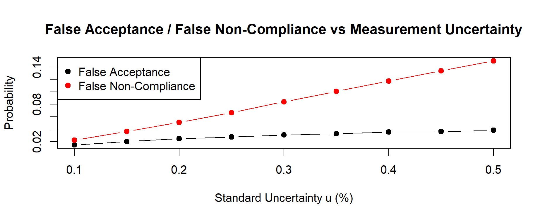
Figure 15.1 – Decision risks of False Acceptance (FA) and False Non-Compliance (FNC) estimated via Monte Carlo uncertainty propagation. Risks increase monotonically with the method-validated standard uncertainty u, showing an asymmetric trade-off driven by the process distribution centered near the upper specification limit (USL = 100%).
Monte Carlo simulation makes this trade-off explicit and quantifiable.
📊 Decision risks at validated MU = 0.25%
False Non-Compliance (FNC) = 0.06798 → 6.80%
(Probability of rejecting a batch that is truly within specification)
False Acceptance (FA) = 0.02817 → 2.82%
(Probability of releasing a batch that is truly out-of-specification)
Minor numerical differences across independent runs are expected due to Monte Carlo sampling variability, even when the underlying process and method uncertainty model remain unchanged.
For all uncertainty levels, the simulation returned the following values:
| u (%) |
False Acceptance (FA) |
False Non-Compliance (FNC) |
| 0.10 |
0.01470 |
0.02216 |
| 0.15 |
0.02017 |
0.03634 |
| 0.20 |
0.02476 |
0.05082 |
| 0.25 |
0.02755 |
0.06672 |
| 0.30 |
0.03062 |
0.08411 |
| 0.35 |
0.03275 |
0.10086 |
| 0.40 |
0.03546 |
0.11740 |
| 0.45 |
0.03627 |
0.13389 |
| 0.50 |
0.03823 |
0.14982 |
These numerical values clearly show that:
– both FA and FNC increase monotonically with the standard uncertainty u;
– FNC is consistently higher than FA, because the process mean is close to the USL.
Monte Carlo simulation quantifies this asymmetry with complete transparency.
Expected pattern:
FA increases with measurement uncertainty (higher risk of releasing bad batches).
FNC also increases (more chance of rejecting good batches).
This mirrors the classical metrology trade-off.
🧭 GMP Interpretation
Key GMP Messages
- Measurement uncertainty cannot be ignored when results are close to specification limits.
- A batch may appear compliant only because of measurement noise.
- Monte Carlo converts MU into quantitative release risk, supporting science-based decisions.
Regulatory alignment
- ICH Q14 — analytical variability, robustness, uncertainty sources
- USP <1220> — uncertainty propagation along the analytical lifecycle
- USP <1210> — interpretation of analytical data
- ISO 17025 / GUM — uncertainty in conformity assessment
Monte Carlo simulation provides a transparent and auditable justification for decisions under uncertainty.
✅ Takeaways
- True value and measured value differ because of measurement uncertainty.
- MU creates two distinct risks: False Acceptance (FA) and False Non-Compliance (FNC).
- Both risks increase with larger MU.
- Monte Carlo simulation quantifies these risks transparently and reproducibly.
- The results support defensible and inspection-ready batch release decisions.
📘 Summary
This case study shows how to combine process variability and measurement uncertainty to quantify regulatory decision risks. Monte Carlo simulation translates MU into concrete probabilities of False Acceptance and False Non-Compliance, supporting modern QRM practices and inspection-ready justification.