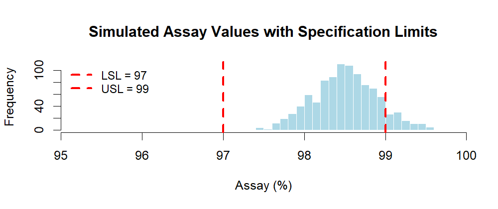
Figure 1.1 – Histogram of simulated assay values with specification limits.
Monte Carlo methods are powerful simulation tools widely used in engineering, finance, and increasingly in the pharmaceutical industry.
In this chapter, you will:
Monte Carlo simulation is a computational method that uses random sampling to estimate numerical results.
It is especially useful when:
The method takes its name from the Monte Carlo Casino in Monaco — a metaphor for randomness, introduced in the 1940s by mathematicians working on complex physics problems. Although originally developed for physics and engineering, Monte Carlo simulation has found increasing relevance in regulated industries such as pharmaceuticals, where uncertainty and variability are central concerns.
In the pharmaceutical and GMP context, Monte Carlo simulation can support a wide range of applications, including but not limited to:
These applications make Monte Carlo not only a statistical curiosity, but a practical decision-support tool for QA, QC, and manufacturing.
Let’s simulate a QC assay that follows a Normal distribution:
set.seed(123)
x <- rnorm(10000, mean = 98.0, sd = 0.4)

# Estimate probability of OOS (out of specification)
mean(x < 97.0 | x > 99.0)
💡 Optional Visualization
Instead of only looking at the calculated OOS risk, we can visualize it.
The histogram below shows 1,000 simulated assay values with specification limits (97% – 99%).
You can clearly see some values falling outside the limits, which matches the estimated OOS probability.
set.seed(123)
x <- rnorm(1000, mean = 98.0, sd = 0.4)
hist(x,
     breaks = 30,
     main = "Simulated Assay Values with Specification Limits",
     xlab  = "Assay (%)",
     col   = "lightblue",
     border= "white",
     xlim  = c(95, 100),
     xaxs  = "i")
abline(v = 97, col = "red", lwd = 3, lty = 2)  # LSL
abline(v = 99, col = "red", lwd = 3, lty = 2)  # USL
legend("topleft", c("LSL = 97", "USL = 99"),
       lty = 2, lwd = 3, col = "red", bty = "n", cex = 0.9)
Figure 1.1 – Histogram of simulated assay values with specification limits.
➡️ What happens here?
We generate 10,000 virtual assay results (like simulating 10,000 potential batches).
We check how many of them fall outside the specifications.
The simulation shows an OOS risk ≈ 0.012 (1.2%). This matches the theoretical calculation using the Normal distribution formula (~1.24%), confirming the accuracy of the Monte Carlo approach.
This simple experiment illustrates the core idea of Monte Carlo:
| ▲ back to top | Next → Random Numbers vs. Random Variates |