Chapter 2 – Random Numbers vs. Random Variates

Monte Carlo simulations require randomness, but not all randomness is the same.
In this chapter, we clarify a crucial distinction:

🎲 Random Numbers

Definition: Numbers generated without a predictable pattern, typically in the range [0, 1].
Source: In practice, they are produced by a pseudo-random number generator (PRNG), which is deterministic but sufficiently random for most statistical simulations.

Example in R:

runif(5)  # Generates 5 random numbers between 0 and 1

Key Point: These are “raw” random values — they are not yet tied to any specific probability distribution.

📈 Random Variates

Definition: Values drawn from a specific probability distribution, obtained by transforming random numbers.
Key Point: Random variates represent real-world data models (e.g., assay values, tablet weights).
Example (conceptual): Transforming random numbers into normally distributed values.

Example in R:

rnorm(5, mean = 100, sd = 15)  # 5 normal variates with mean 100, sd 15

📦 Concept Box – Variability vs Uncertainty

Concept	Definition	Pharmaceutical Example	Reducible?
Variability (aleatory, intrinsic)	Real differences between units or events, part of the system itself.	Weight of 100 tablets from the same batch: values will never be identical, even in a stable process.	❌ Not by measuring more, only by improving the process.
Uncertainty (epistemic, knowledge-based)	Lack of knowledge about the true value of a parameter or about the model.	We do not know exactly the true standard deviation of tablet weights; we estimate it from a sample.	✅ Yes, by collecting more data or refining the model.

Practical Note

Variability = what really makes units differ from each other.
Uncertainty = what makes us unsure about the system’s parameters.
Variability is modeled by probability distributions (e.g., Normal for tablet weights).
Uncertainty is modeled by distributions on parameters (e.g., Beta for defect probability, bootstrap for variance).

🔄 From Numbers to Variates

Figure 2.1 – Random Numbers to Random Variates
Figure 2.1 – Transformation process: from raw uniform random numbers to model-based random variates.

Generate uniform random numbers.
Apply a transformation (inverse CDF or algorithm) to match the target distribution.
Obtain random variates that reflect the desired model.

Example in R – Transforming Uniform → Normal

u <- runif(1000)
x <- qnorm(u, mean = 50, sd = 5)

hist(x,
     main = "Normal Variates from Uniform Random Numbers",
     xlab = "Value",
     col = "lightblue",
     border = "white")

➡️ What happens here?

We first generate 1,000 uniform random numbers between 0 and 1.
We then apply the inverse Normal CDF (qnorm) to transform them into values that follow a Normal distribution (mean = 50, sd = 5).
The histogram shows that the values now follow the familiar bell-shaped curve.

🔎 Note – What is the inverse Normal CDF?
The inverse Normal CDF (also called the quantile function) tells us:
“Given a probability p, which value x of the Normal distribution has that cumulative probability?”
For example, the 0.975 quantile of a standard Normal distribution is 1.96 — meaning 97.5% of values lie below 1.96.

This demonstrates the core idea:

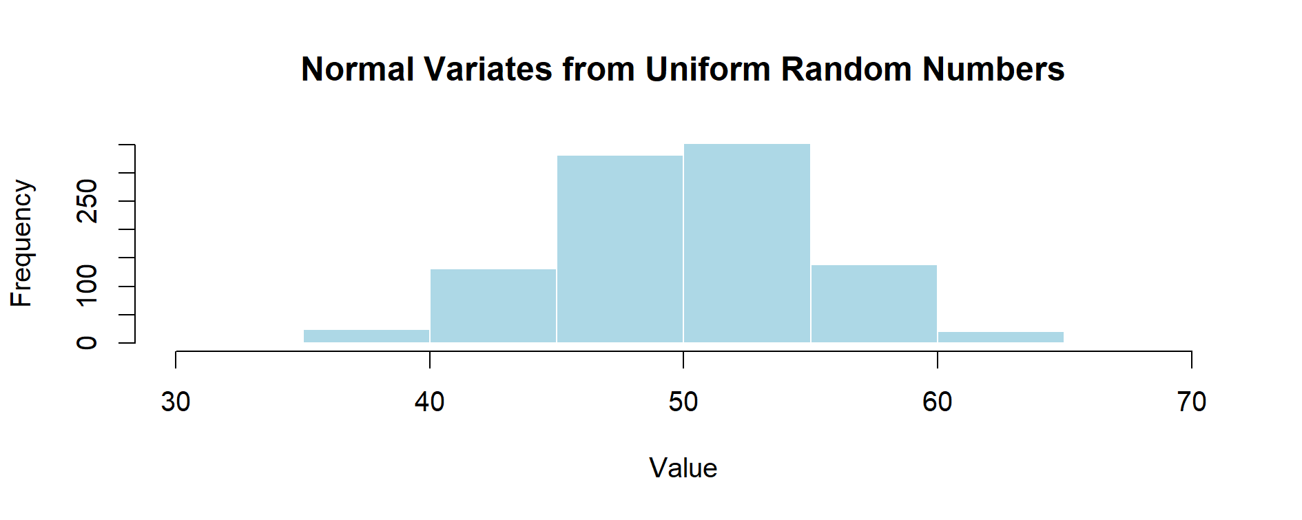
Uniform random numbers are the raw material.
Random variates are shaped into a distribution that models real-world phenomena (e.g., tablet weight around 50 mg).

Figure 2.2 – Transforming Uniform Random Numbers into Normal Variates (mean = 50, sd = 5).

📌 Historical Note — Random Numbers vs Random Variates
In early simulation texts (e.g., Rubinstein, 1981), the term random numbers was often used broadly, referring both to

uniform sequences U(0,1), and

sampled values from target distributions.

Modern usage (2025) makes a clearer distinction:

Random numbers = pseudorandom draws ∼ U(0,1),

Random variates = transformed values from those numbers (e.g., inversion, Box–Muller, rejection).

This two-step view is pedagogically useful: it emphasizes that every random variate is ultimately built on top of uniform random numbers.

📊 Random Numbers vs Random Variates — Rubinstein (1981) vs Modern View (2025)

Aspect	Rubinstein (1981)	Modern View (2025)
Terminology	Uses random numbers broadly, covering both uniforms and variates	Clear separation: numbers = U(0,1), variates = transformed values
Definition of numbers	“Independent random variables uniformly distributed over [0,1]” (p. 11)	Numbers from a PRNG, ideally i.i.d. U(0,1)
Definition of variates	Mentions “stochastic variates” but without stressing the intermediate role of uniforms	Explicit: variates are generated from uniform numbers via inversion, Box–Muller, rejection
Pedagogical clarity	Implicit two-step process assumed	Two distinct layers emphasized for teaching
Example	Sampling directly from exponential or normal without detailing the uniform step	Example: U∼U(0,1); X = -λ⁻¹ ln(1-U) → exponential variate
Why the difference?	Terminology less standardized; focus on algorithms	Modern pedagogy highlights the distinction for clarity

💊 Why It Matters in Pharma

In pharmaceutical applications:

Random Numbers simulate uncertainty in a general sense, without context.
Random Variates simulate actual process or measurement data (e.g., tablet weight, assay results).
Using the wrong one may lead to unrealistic or misleading outcomes.

👉 This distinction is fundamental: all Monte Carlo simulations in GMP contexts are ultimately based on random variates, not raw random numbers.
This foundation is essential for moving forward. In the next chapter, we will explore the most common probability distributions used in pharmaceutical applications.

← Previous: Introduction

▲ back to top

Next → Simple Distributions