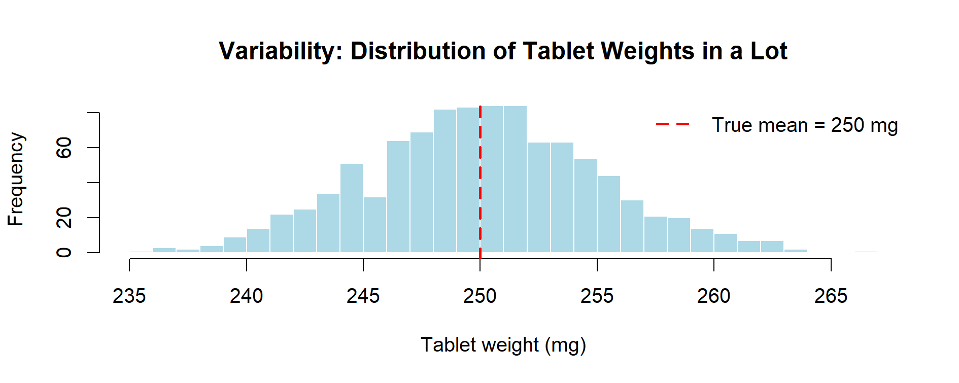
Figure 5.1 – Variability: distribution of tablet weights in a simulated lot (1,000 tablets). The spread around the true mean (250 mg) represents intrinsic variability of the process.
In the previous chapter we introduced the concept of the transfer equation and showed how inputs and outputs can be mathematically linked. That was a first illustrative step, sufficient to understand the logic but intentionally limited in scope.
Now we take a real leap forward: in this chapter we combine random variates, input distributions, and the transfer equation into a complete Monte Carlo simulation. This is the first full example, where we do not only define the model but also generate thousands of realizations, visualize the results, and interpret them in terms of pharmaceutical specifications.
Before running our first complete Monte Carlo simulation, it is useful to clarify the difference between variability and uncertainty with a simple visual experiment.
set.seed(123)

# --- Variability: tablet weights from a given process ---
true_mean <- 250     # mg
true_sd   <- 5       # mg
n_lot     <- 1000    # tablets in a lot

# Simulated lot: represents intrinsic variability
lot_weights <- rnorm(n_lot, mean = true_mean, sd = true_sd)

# --- Uncertainty: estimating the mean from a small sample ---
n_sample <- 20
sample_weights <- sample(lot_weights, n_sample)

mean_est <- mean(sample_weights)
sd_est   <- sd(sample_weights)

# Confidence interval for the true mean (uncertainty in estimation)
ci <- t.test(sample_weights)$conf.int

list(
  estimated_mean = mean_est,
  estimated_sd   = sd_est,
  CI_for_mean    = ci
)

# --- Plot 1: Variability (histogram of lot weights) ---
hist(lot_weights,
     breaks = 30,
     col = "lightblue",
     border = "white",
     main = "Variability: Distribution of Tablet Weights in a Lot",
     xlab = "Tablet weight (mg)")
abline(v = true_mean, col = "red", lwd = 2, lty = 2)
legend("topright", legend = c("True mean = 250 mg"),
       col = "red", lty = 2, lwd = 2, bty = "n")

# --- Plot 2: Uncertainty (sample mean with 95% CI) ---
plot(1, mean_est,
     ylim = c(true_mean - 5, true_mean + 5),   # wider margin
     pch = 19, col = "blue",
     xlab = "", ylab = "Estimated mean weight (mg)",
     xaxt = "n",
     main = "Uncertainty: Mean Estimate from 20 Tablets")

arrows(1, ci[1], 1, ci[2],
       angle = 90, code = 3, length = 0.1,
       col = "blue", lwd = 2)

abline(h = true_mean, col = "red", lwd = 2, lty = 2)

legend("bottomright",
       legend = c("True mean = 250 mg", "Sample mean ± 95% CI"),
       col = c("red","blue"),
       lty = c(2,1), pch = c(NA,19),
       lwd = c(2,2), bty = "n")
Figure 5.1 – Variability: distribution of tablet weights in a simulated lot (1,000 tablets). The spread around the true mean (250 mg) represents intrinsic variability of the process.
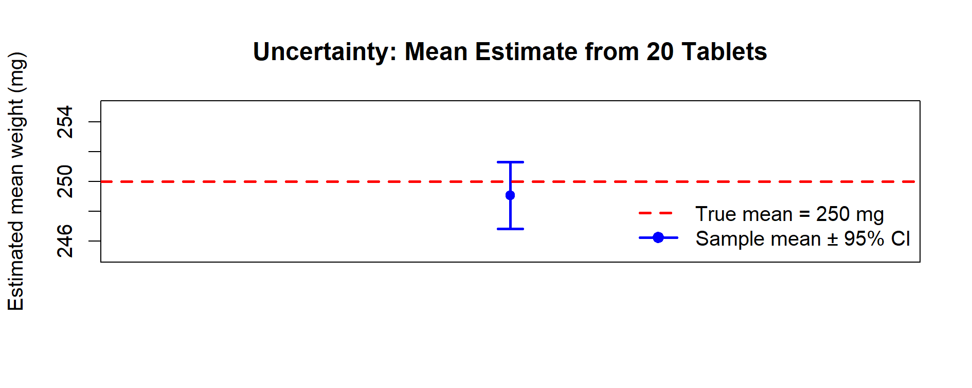
Figure 5.2 – Uncertainty: estimate of the mean from a sample of 20 tablets. The point estimate is shown with its 95% confidence interval. The dashed red line is the true mean (250 mg).
We want to simulate the assay of a tablet to assess if the process meets specifications:
LSL = 98.0%, USL = 102.0%.
Inputs:
API_weight → Normally distributed (mean = 101 mg, sd = 2 mg)Tablet_weight → Normally distributed (mean = 250 mg, sd = 5 mg)Purity → Uniform distribution (min = 0.98, max = 1.00)Transfer Equation (normalized to the label claim = 100 mg):
Assay(%) = (API_weight * Purity / LabelClaim) * 100 (with LabelClaim = 100 mg)
👉 Note: Tablet_weight is generated here as an example of an additional variable that could be used in extended scenarios (e.g., content uniformity). In this basic example it is not directly part of the assay formula.
set.seed(123)

# 1) Number of simulations
N <- 10000

# 2) Random inputs (as in the scenario)
API_weight    <- rnorm(N, mean = 101, sd = 2)          # raw API mass
Tablet_weight <- rnorm(N, mean = 250, sd = 5)          # not used here, but useful for extensions
Purity        <- runif(N, min = 0.98, max = 1.00)      # purity fraction

# 3) Transfer equation normalized to the API's Label Claim
LabelClaim <- 100                                       # mg
Assay <- (API_weight * Purity / LabelClaim) * 100       # % respect to the Label Claim

# 4) Summary
cat("Summary of Assay %:\n")
print(summary(Assay))
cat("Standard Deviation:", sd(Assay), "\n")

# 5) Histogram + specification limits
hist(Assay,
     main = "Simulated Assay (%)",
     xlab = "Assay %",
     col = "lightblue",
     border = "white")
abline(v = c(98, 102), col = "red", lwd = 2, lty = 2)

# 6) Q-Q plot
qqnorm(Assay, main = "Q-Q Plot of Simulated Assay")
qqline(Assay, col = "red", lwd = 2)

# 7) Quantiles
qs <- quantile(Assay, probs = c(0, .25, .5, .75, 1))
IQR_val <- unname(qs[4] - qs[2])

cat(sprintf(
  "Mean=%.2f, SD=%.2f, Min=%.2f, Q1=%.2f, Median=%.2f, Q3=%.2f, IQR=%.2f, Max=%.2f, OOS=%.2f%%\n",
  mean(Assay), sd(Assay), qs[1], qs[2], qs[3], qs[4], IQR_val, qs[5], 100*mean(Assay < 98 | Assay > 102)
))

# 8) Probability of OOS
p_out <- mean(Assay < 98 | Assay > 102)
cat("Probability out of spec:", p_out, "\n")
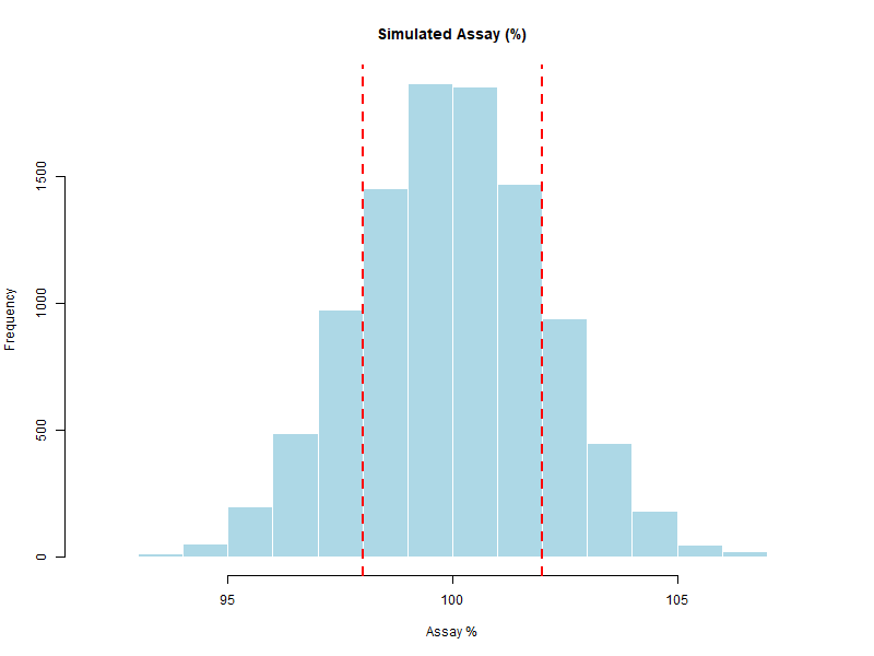
Figure 5.3 – Histogram of simulated assay values with specification limits
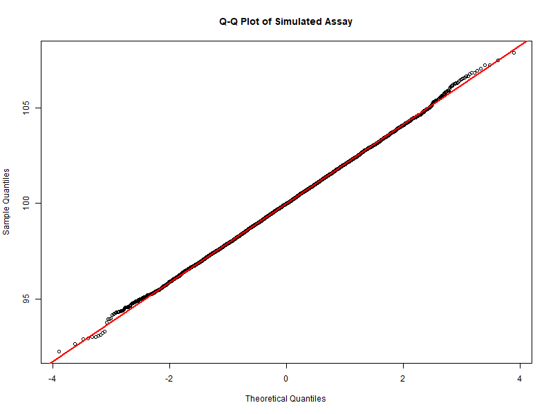
Figure 5.4 – Q-Q Plot of simulated assay values
p_out → probability of being out of specification| Statistic | Value |
|---|---|
| Mean Assay (%) | 99.98 |
| Median Assay (%) | 99.98 |
| SD | 2.06 |
| Min | 92.27 |
| Q1 (25th) | 98.59 |
| Q3 (75th) | 101.38 |
| IQR | 2.79 |
| Max | 107.87 |
| Probability OOS | 33.58% |
Note: Exact numbers may vary slightly due to random simulation,
but results are reproducible with the fixed seed (set.seed(123)).
This simulation provides more than a single result:
p_out) directly expresses the risk of producing tablets outside the 98–102% range.If p_out is very low (e.g., < 0.1%), the process is highly capable.
If p_out is significant, we may need to:
👉 In GMP contexts, such probabilities (p_out) directly inform risk-based decisions: whether the process can be accepted, requires corrective actions, or must be redesigned.
In the next chapter we will systematically analyze these results, introducing graphical summaries and capability indices to turn raw Monte Carlo output into structured GMP insights.
| ← Previous: The Transfer Equation | ▲ back to top | Next → Analysis of Results |