Chapter 7 — Case Study 1 — API Assay in Tablets

In this chapter, we present a realistic GMP pharmaceutical example to demonstrate the complete Monte Carlo workflow — from defining inputs to interpreting results.

💊 Scenario: Assay of an API in Finished Tablets

A Quality Control laboratory is validating a new process for producing tablets containing an Active Pharmaceutical Ingredient (API).
The target assay is 100.0% with specifications:

• LSL = 98.0%
• USL = 102.0%

📥 Step 1 – Define Inputs and Distributions

Based on historical data and expert estimates:

Note: “API Label Claim” refers to the declared API content (mg), not the total tablet mass.

🔗 Step 2 – Define the Transfer Equation

The assay is calculated using the ratio of API weight to API label claim, multiplied by purity and converted to a percentage:

Assay(%) = (API_weight / API_LabelClaim) * Purity * 100

Note: “API Label Claim” represents the declared API content per tablet (mg), used as the denominator in the transfer equation. It does not refer to the total tablet mass.

💻 Step 3 – Run the Simulation in R

set.seed(123)

# Number of simulations
N <- 100000

# NOTE ON VARIABLES:
# - API_weight: measured API content per tablet (mg)
# - API_LabelClaim: declared API content (mg), not total tablet mass
# - Purity: assay purity (fraction), used as correction factor

# 1) Random inputs (choose realistic values so that assay ~ 100%)
API_weight    <- rnorm(N, mean = 100.5, sd = 1.2)  # mg measured API
API_LabelClaim <- rnorm(N, mean = 100.0, sd = 0.5)  # mg label claim (API)
Purity        <- runif(N, min = 0.985, max = 1.000)

# 2) Transfer equation
Assay <- (API_weight / API_LabelClaim) * Purity * 100

# Quick sanity-check on center and spread
mean_assay <- mean(Assay)
sd_assay   <- sd(Assay)

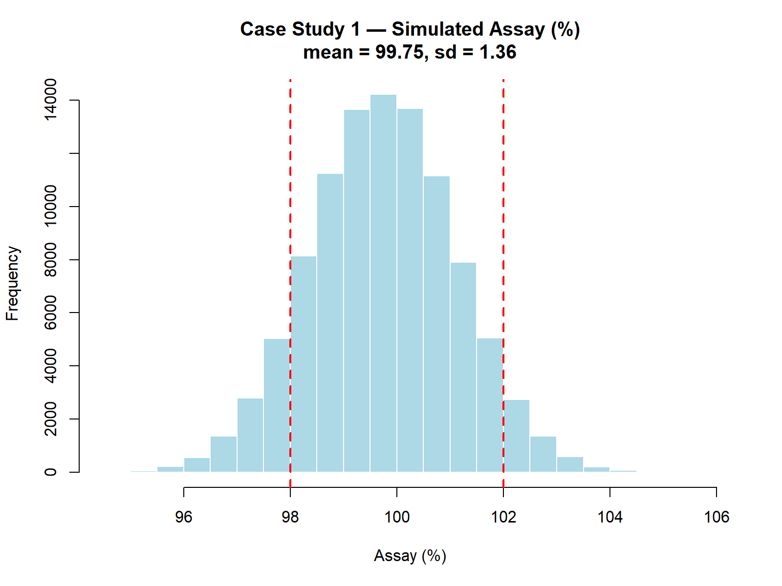
# 3) Histogram with specs
hist(Assay, 
     main = sprintf("Case Study 1 — Simulated Assay (%%) — mean=%.2f, sd=%.2f", mean_assay, sd_assay),
     xlab = "Assay (%)",
     col = "lightblue",
     border = "white")
abline(v = c(98, 102), col = "red", lwd = 2, lty = 2)

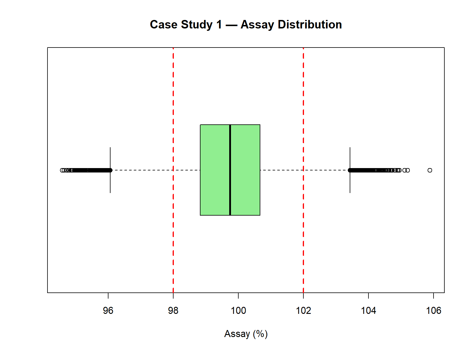
# 4) Boxplot
boxplot(Assay, horizontal = TRUE,
        main = "Case Study 1 — Assay Distribution",
        col = "lightgreen")
abline(v = c(98, 102), col = "red", lwd = 2, lty = 2)

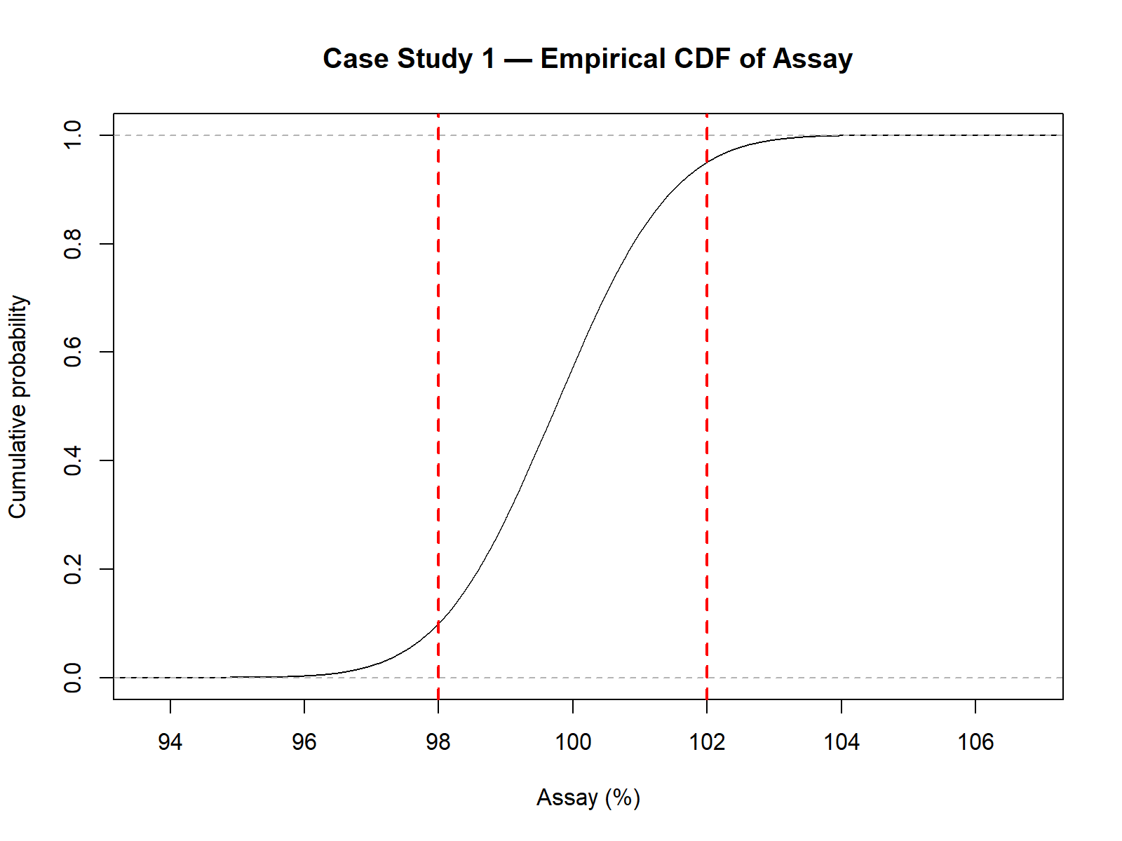
# 5) ECDF
plot(ecdf(Assay),
     main = "Case Study 1 — Empirical CDF of Assay",
     xlab = "Assay (%)",
     ylab = "Cumulative probability")
abline(v = c(98, 102), col = "red", lwd = 2, lty = 2)

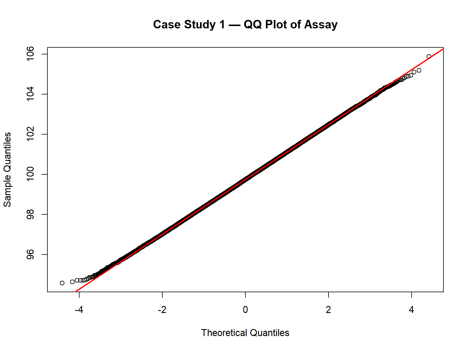
# 6) QQ plot for normality check
qqnorm(Assay, main = "Case Study 1 — QQ Plot of Assay")
qqline(Assay, col = "red", lwd = 2)

# 7) Probability of OOS
p_out <- mean(Assay < 98 | Assay > 102)

# 8) Capability index vs 98–102 (normality assumption)
USL <- 102; LSL <- 98
Cpk <- min((USL - mean_assay) / (3 * sd_assay),
           (mean_assay - LSL) / (3 * sd_assay))

list(mean_assay = mean_assay, sd_assay = sd_assay, p_out = p_out, Cpk = Cpk)

📊 Step 4 – Example Output

• Histogram with red dashed lines marking specification limits.
• Observed results for this simulation:
  • Mean assay: 99.75%
  • Standard deviation: 1.36%
  • Probability of OOS (p_out): 14.95%
  • Cpk: ≈ 0.43 → far below the GMP-recommended threshold of 1.33

Summary of simulated assay results (N = 100,000):

These values indicate a process with excessive variability and a non-negligible risk of producing batches outside specifications.

Note: This dataset was chosen deliberately to illustrate how Monte Carlo simulations can reveal a process that is not in control.
In a real GMP context, results like these would trigger a root cause investigation and corrective actions to reduce variability and improve process centering.

Cpk was calculated as:

Cpk = min( (USL - μ)/(3*σ), (μ - LSL)/(3*σ) )

Note: The closed-form Cpk assumes approximate normality. For skewed or non-normal data, percentile-based indices or Monte Carlo percentiles are more robust. In GMP reports, it is often recommended to present both parametric indices (like Cpk) and percentile-based indices,
to ensure robustness against deviations from normality.

📌 Step 5 – GMP Interpretation

• High p_out (~15%): significant risk of non-compliance.
• Low Cpk (~0.43): process poorly centered and/or with high variability.
• Immediate corrective and preventive actions (CAPA) would be needed before routine production.

Reminder: Unlike the “ideal” scenarios shown earlier (low p_out, high Cpk),
this case study was selected to demonstrate how Monte Carlo simulation can highlight an at-risk process and guide GMP decision-making.

This approach can be extended to future case studies, such as:

• Dissolution testing
• Content uniformity
• Stability data projections
• Microbiological limits

This quantitative approach supports risk-based decision-making and can be documented in validation or continued process verification reports.

🔄 Step 6 – What-if Scenario (Process Improvement)

Suppose variability of API weight is reduced from sd = 1.2 mg → sd = 0.8 mg
(e.g., by better control of blending and compression).

Re-running the simulation (after process improvement, N = 100,000) yields:

Comparison: Before vs After Process Improvement

This demonstrates how Monte Carlo can quantify the benefit of CAPA actions,
providing objective evidence that process improvements significantly reduce the risk of non-compliance.

🔎 Regulatory Note:
This type of Monte Carlo analysis aligns with the ICH Q9(R1) principles of risk management,
and can support documentation in Process Validation Stage 3 (Continued Process Verification)
as recommended in FDA and EMA guidelines.

These results illustrate how Monte Carlo simulation provides not only descriptive statistics, but also probabilistic evidence of compliance risk,
which can be directly incorporated into GMP decision-making and regulatory documentation.

In the next chapter, we expand this perspective by showing how simulation results can systematically support decision-making and risk management in GMP contexts.