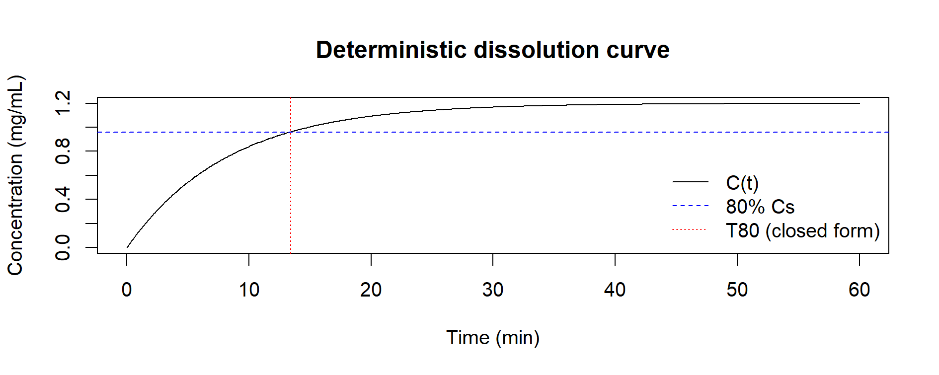
Figure 8.1 – Deterministic dissolution curve using the Noyes–Whitney model (k = 0.12, Cs = 1.20 mg/mL). The dashed line marks 80% Cs, the dotted line the T80 closed-form solution (≈13 min).
In this chapter, we illustrate how Monte Carlo methods can be applied to dissolution testing,
a critical parameter in pharmaceutical development and quality control.
We contrast:
📌 Monte Carlo and Two Classes of Problems
As emphasized already in early texts (e.g. Hammersley & Handscomb, 1964), Monte Carlo methods can be applied to two broad classes of problems:
Probabilistic problems
These are problems that are intrinsically random, where the Monte Carlo method simulates the underlying stochastic process.
Examples: growth of insect populations, traffic in telephone exchanges, neutron diffusion in reactors.Deterministic problems
These are problems that are not random in themselves, but can be reformulated in probabilistic terms.
The Monte Carlo method then solves the equivalent random problem to obtain the answer to the original deterministic one.
Examples: numerical solutions of differential equations such as Laplace or Schrödinger, or—here—dissolution kinetics.This distinction remains pedagogically useful today: Monte Carlo is not limited to probability theory.
It also provides an alternative, variability-oriented lens on deterministic models, enriching their interpretation.
Dissolution testing evaluates the rate at which an Active Pharmaceutical Ingredient (API) dissolves in a medium.
The Noyes–Whitney law provides a simple first-order differential equation for drug concentration over time:
Where:
A key metric is T80: the time required to reach 80% of solubility.
📘 Historical Note – The Noyes–Whitney Law (1897)
The Noyes–Whitney equation describes dissolution as a first-order differential equation.The model assumes that the dissolution rate is proportional to the difference between saturation concentration and current concentration.
While today more complex models exist (e.g. Nernst–Brunner, diffusion layer models), Noyes–Whitney remains:
- mathematically simple,
- analytically solvable (closed-form solution exists),
- and therefore highly suitable for didactic demonstration.
In this case study, it serves as an ideal example of a deterministic problem (a first-order ODE with known solution)
that can also be explored via Monte Carlo simulation, showing how parameter variability leads to a distribution of outcomes.
We first simulate dissolution using fixed parameters:
# Deterministic simulation (Euler method)
k   <- 0.12      # 1/min
Cs  <- 1.20      # mg/mL
C0  <- 0         # mg/mL
t_end <- 60      # minutes
dt    <- 0.1
time  <- seq(0, t_end, by=dt)

C <- numeric(length(time))
C[1] <- C0
for (i in 2:length(time)) {
  dCdt <- k * (Cs - C[i-1])
  C[i] <- C[i-1] + dt * dCdt
}

target <- 0.80 * Cs
i_hit  <- which(C >= target)[1]
T80_closed <- log(5) / k   # closed-form check

# --- Plot the dissolution curve ---
plot(time, C,
     type = "l",
     xlab = "Time (min)",
     ylab = "Concentration (mg/mL)",
     main = "Deterministic dissolution curve")

# Add horizontal line for 80% Cs
abline(h = target, lty = 2, col = "blue")

# Add vertical line for T80 (closed form)
abline(v = T80_closed, lty = 3, col = "red")

legend("bottomright",
       legend = c("C(t)", "80% Cs", "T80 (closed form)"),
       lty = c(1, 2, 3),
       col = c("black", "blue", "red"),
       bty = "n")
Figure 8.1 – Deterministic dissolution curve using the Noyes–Whitney model (k = 0.12, Cs = 1.20 mg/mL). The dashed line marks 80% Cs, the dotted line the T80 closed-form solution (≈13 min).
The deterministic model yields a single estimate of T80 (≈ 13 min).
In practice, dissolution parameters vary due to formulation, medium, temperature, and other experimental factors. We model uncertainty as:
We then simulate 5,000 virtual experiments.
set.seed(123)
N <- 5000

# Helper to sample lognormal from mean & CV
r_lognorm_from_mean_cv <- function(n, mean, cv){
  sigma2 <- log(1 + cv^2)
  mu     <- log(mean) - 0.5*sigma2
  rlnorm(n, meanlog = mu, sdlog = sqrt(sigma2))
}

k_samp  <- r_lognorm_from_mean_cv(N, mean=0.12, cv=0.25)
Cs_raw  <- rnorm(N, mean=1.20, sd=0.05)
Cs_samp <- ifelse(Cs_raw > 0, Cs_raw, 1.20)

# Quantity of interest: T80 = ln(5)/k
T80 <- log(5) / k_samp

mean_T80 <- mean(T80)
sd_T80   <- sd(T80)
ci_T80   <- mean_T80 + c(-1,1) * qt(0.975, df=N-1) * sd_T80/sqrt(N)
p_T80_30 <- mean(T80 <= 30)

# --- Plot 1: Distribution of T80 ---
hist(T80,
     breaks = 40,
     xlab = "T80 (min)",
     main = "Distribution of T80 (Monte Carlo)",
     col = "lightblue",
     border = "white")
abline(v = mean_T80, col = "red", lwd = 2, lty = 2)
legend("topright",
       legend = c(sprintf("Mean = %.2f", mean_T80),
                  sprintf("95%% CI = [%.1f, %.1f]", ci_T80[1], ci_T80[2])),
       bty = "n")

# --- Plot 2: Fan of dissolution curves C(t) ---
time <- seq(0, 60, by = 0.5)
ns <- 20
idx <- sample(seq_len(N), ns)

matplot(time,
        sapply(idx, function(j) Cs_samp[j] * (1 - exp(-k_samp[j] * time))),
        type = "l", lty = 1, col = "gray",
        xlab = "Time (min)", ylab = "Concentration (mg/mL)",
        main = "Monte Carlo fan of dissolution curves")
abline(h = 0.8 * mean(Cs_samp), lty = 2, col = "blue")
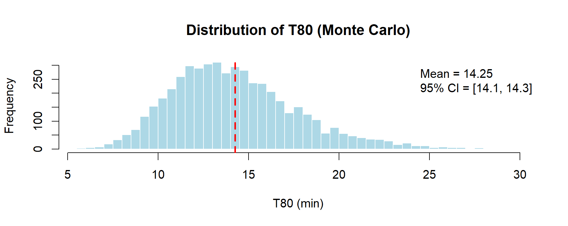
Figure 8.2 – Distribution of T80 values obtained by Monte Carlo simulation (N = 5000). The variability in k leads to a spread of dissolution times, though all below 30 min.
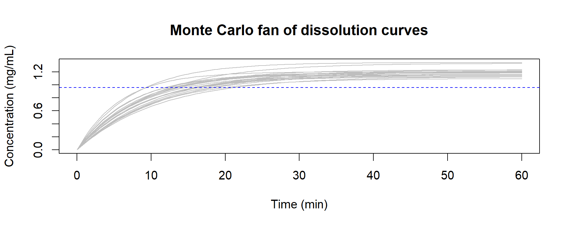
Figure 8.3 – Example of 20 dissolution curves simulated via Monte Carlo (random draws of k and Cs). The fan of profiles illustrates process variability around the deterministic expectation.
The Empirical Cumulative Distribution Function (ECDF) of T80 allows a direct read of probabilities (e.g. % of cases below 30 min).
plot(ecdf(T80),
     main = "ECDF of T80 (Monte Carlo)",
     xlab = "T80 (min)",
     ylab = "Cumulative probability",
     col = "blue", lwd = 2)
abline(v = 30, col = "red", lty = 2)
abline(h = p_T80_30, col = "red", lty = 2)

legend("bottomright",
       legend = c(sprintf("P(T80 ≤ 30) = %.1f%%", 100*p_T80_30)),
       col = "red", lty = 2, bty = "n")
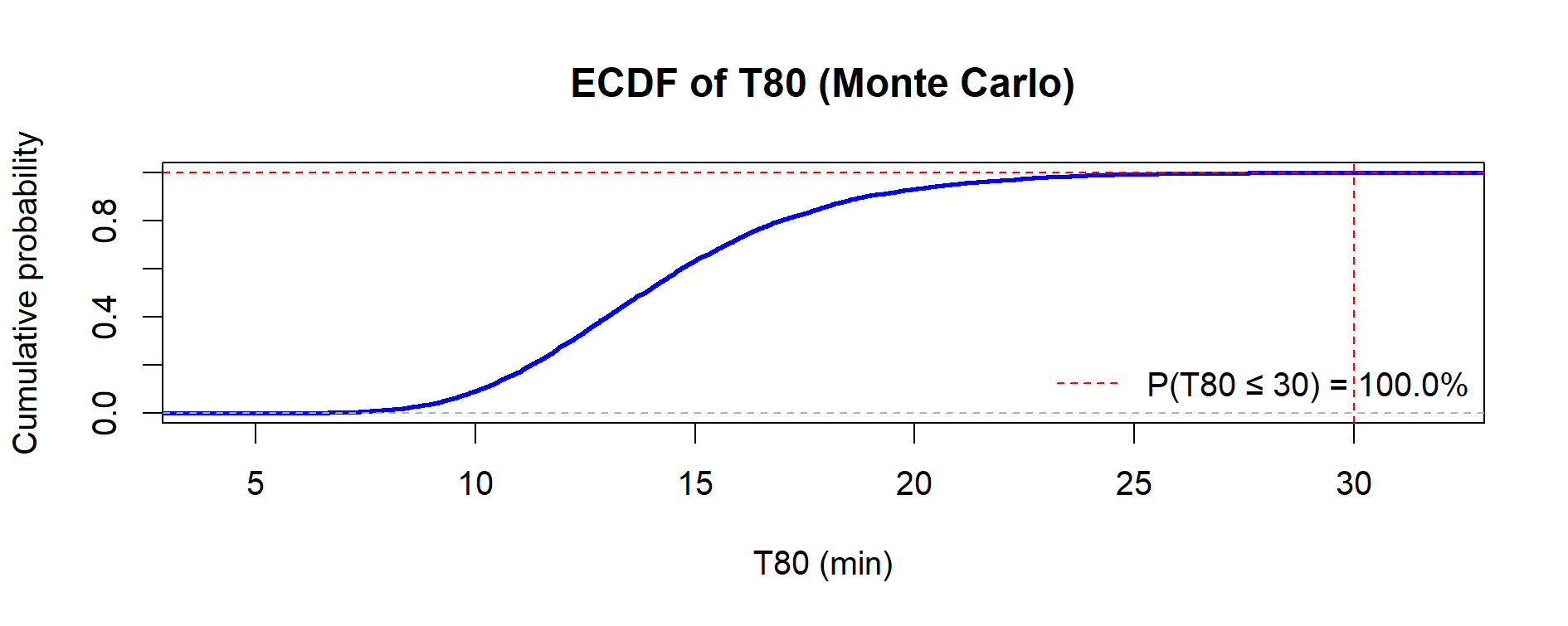
Figure 8.4 – ECDF of simulated T80 values (N = 5,000). The vertical line marks 30 min; the horizontal line shows that 100% of cases fall below this threshold.
Summary statistics (N = 5,000):
| Statistic | Value |
|---|---|
| Mean T80 (min) | ≈13.5 |
| Standard deviation (SD) | ≈3.0 |
| 95% Confidence Interval for T80 (min) | ≈[7.7, 19.3] min |
| Probability T80 ≤ 30 min | 100% |
In probabilistic terms, the Monte Carlo estimate of P(T80 ≤ 30 min) = 1.00 represents a quantitative confirmation of compliance,
showing that even under parameter uncertainty the process operates with negligible risk of failure.
Regulatory Note:
Monte Carlo analysis of dissolution is consistent with ICH Q9(R1) (risk management) and USP <1210> (simulation as supportive tool).
It provides a richer picture than single deterministic estimates, making risk-based decisions more transparent.
| ← Previous: Case Study 1 — API Assay in Tablets | ▲ Back to top | Next: Case Study 3 — From 3 Batches to Continuous Confidence → |